Spreadsheets Extension for Qlik Sense

Downloading and Installing

Qlik Sense Desktop

To install Spreadsheets Extension in Qlik Sense Desktop, do the following:

1. Download Spreadsheets Extension for Qlik Sense.
2. Extract the archive.
3. Open a Windows Explorer window and navigate to the Qlik Sense Extensions directory: ..\Users\<UserName>\Documents\Qlik\Sense\Extensions.
4. Copy the anychart–4x–spreadsheets folder to the Extensions directory.
5. Relaunch Qlik Sense Desktop.

Qlik Sense Server

To install Spreadsheets Extension on a Qlik Sense server,

1. Download Spreadsheets Extension for Qlik Sense.
2. Open Qlik Management Console (QMC): https://<QPS server name>/qmc
3. Select Extensions on the QMC start page or from the Start drop–down menu.
4. Click Import in the action bar.
5. In the dialog, select the downloaded archive. Leave the password area blank.
6. Click Open in the file explorer window.
7. Click Import.

Qlik Sense Cloud

To install Spreadsheets Extension in Qlik Sense Cloud, do the following:

1. Download Spreadsheets Extension for Qlik Sense Cloud.
2. Extract the archive.
3. Access the Management Console:
   • add /console to your tenant address: https://<your tenant address>/console
   • or use the navigation link Administration under the user profile in the hub
4. Go to the Extensions page and click Add.
5. In the dialog, select the archive with the extension in the bundle — for example, anychart–4x–spreadsheets.zip.
6. Click Add.
7. Repeat the steps above to add other extensions.
8. In the Management Console, go to the Content Security Policy section and click Add.
9. In the dialog, give the Content Security Policy a name — for example, AnyChart.
10. Type the address of the origin server: qlik.anychart.com
11. Select the following directives:
    • connect–src
    • font–src
    • img–src
    • script–src
    • style–src
12. Click Add.

Overview

AnyChart Spreadsheets brings a powerful, Excel–like table editing experience directly into Qlik Sense. With support for native Excel formulas, rich formatting, multi–sheet setups, and interactive data exploration, this extension enables users to manipulate and analyze data with the flexibility of a full–featured spreadsheet.

Explore the Quick Start section to get hands–on experience on the Spreadsheets extension.

Quick Start

Create a Basic Table

This tutorial walks you through creating a basic Spreadsheets visualization from scratch.

Video walkthrough:

Step 1: Add an Empty Visualization

1. In your Qlik Sense app, go to the Assets Panel.
2. Navigate to Custom objects > AnyChart 4.
3. Drag the Spreadsheets Table visualization onto your sheet.

Step 2: Add a Data Section

1. Select the visualization and open the Properties Panel.
2. Go to the Data section.
3. Click the Add button to create a new Data Section.
4. Select the newly created Data Section.
5. Ensure the Create synced sheet toggle is turned on.
6. Click Edit data and select Data.
7. Add your desired Dimensions and Measures.

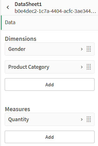
After completing these steps, your visualization will contain:

• One empty sheet: Sheet1
• One data–populated sheet from the Data Section: DataSheet1

Step 3: Format the Spreadsheet

Remove the empty sheet:

1. Right–click on Sheet1 and select Delete.

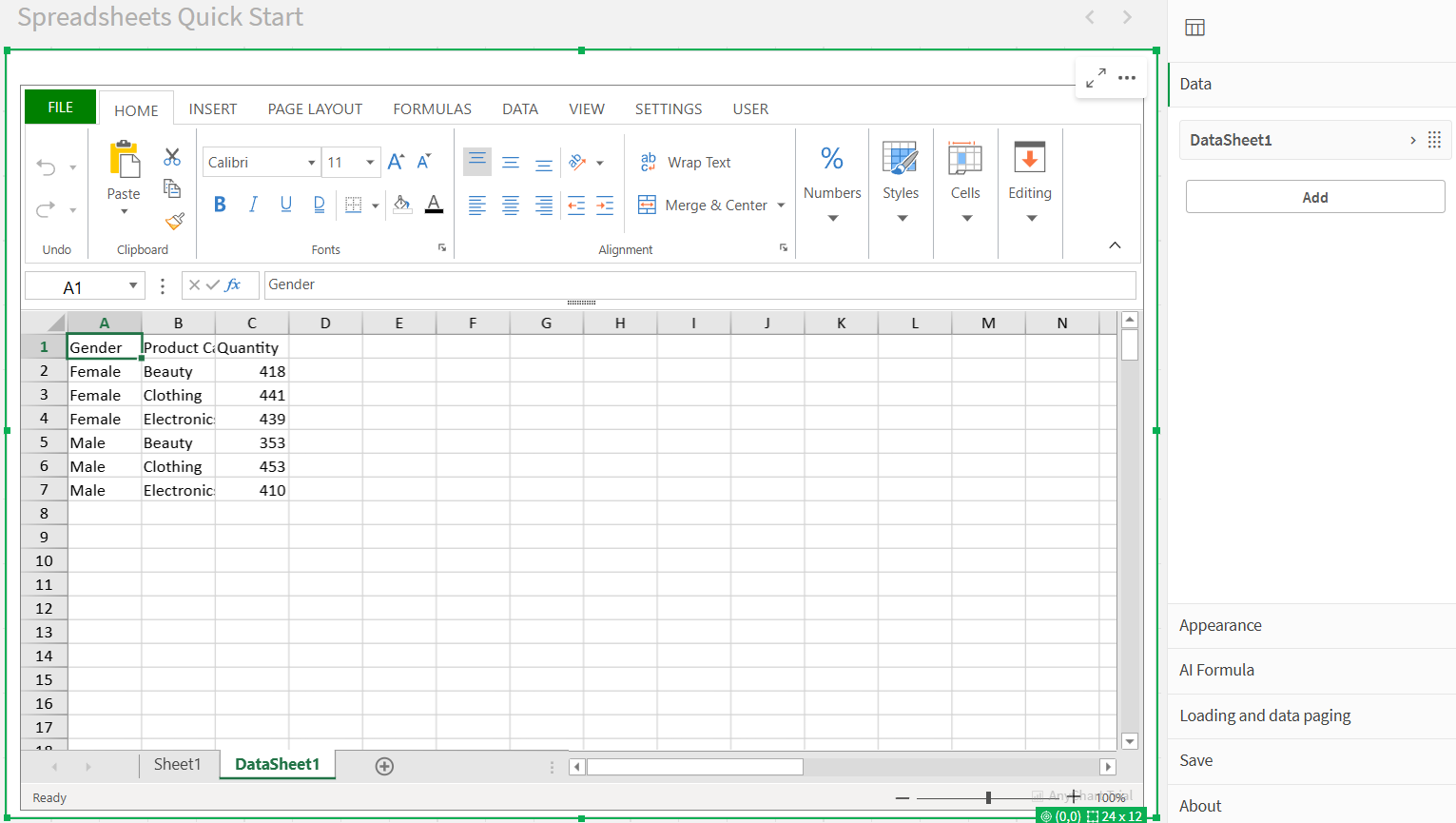
Create a table on the remaining data sheet:

1. Select all cells containing data.
2. Go to the INSERT section in the Ribbon Menu.
3. Click Table, then confirm in the pop–up window.

Adjust formatting:

1. Resize columns and rows as needed.
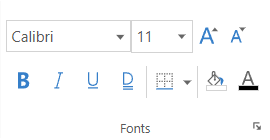
2. Customize font styles using the HOME tab.
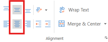
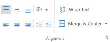
3. Select your header cells and use alignment tools under Font Alignment.

Step 4: Add a Chart

1. Select all cells containing data.
2. Go to the INSERT tab in the Ribbon Menu.
3. Click Insert Chart and choose a chart type that fits your data.
4. Click OK. Reposition your chart anywhere on the sheet.

Step 5: Save Your Changes

1. Go to the USER tab in the Ribbon Menu.
2. Click Save to app.
3. Confirm the save action in the pop-up window.

At this point, you've built a basic spreadsheet visualization fully integrated with your Qlik data. It can now be used, shared, or extended further.

Optional: Export Your Spreadsheet to Excel

If you want to continue working in another tool like Excel:

1. Go to the FILE tab in the Ribbon Menu.
2. Click Export.
3. Select the Excel file option.
4. Configure your export settings using Save Flags.
5. Click the Export Excel File button.
6. Name your file in the pop-up window and click OK.

After that, the download will start automatically, and your .xlsx file will be ready to open in Excel or any compatible software.

Use existing excel template

This guide walks you through how to use the AnyChart Spreadsheets extension in Qlik Sense to turn an Excel template into a fully interactive, data–driven spreadsheet.

Video walkthrough:

Prerequisites

• Qlik Sense app with the AnyChart Spreadsheets extension installed.
• Template file: personal–budget.xlsx

Step 1: Load Data into Qlik

1. Upload the personal–budget.xlsx file to the Attached Files of your Qlik app.
2. Open the Data Load Editor and use the following script to load the Budget and Transactions tables:

   
   LOAD
     Category,
     Amount
   FROM [lib://AttachedFiles/personal–budget.xlsx]
   (ooxml, embedded labels, header is 3 lines, table is Budget)
   Where Upper(Trim(Category)) <> 'TOTAL';
   
   LOAD
     "Date",
     Description,
     Category,
     Amount
   FROM [lib://AttachedFiles/personal–budget.xlsx]
   (ooxml, embedded labels, header is 1 line, table is Transactions);
             

3. Click Load Data.

Step 2: Add the Spreadsheets Extension

1. Create a new sheet in your Qlik app and open it. Enter Edit Mode.
2. From the Custom Objects > AnyChart section, drag the Spreadsheets Table visualization onto the canvas.

Step 3: Import the Excel Template

1. With the visualization selected, go to the FILE tab in the ribbon menu.
2. Click Import Excel File.
3. Select the personal–budget.xlsx file.

The template contains two sheets:

• A Budget sheet
• A Transactions sheet

Step 4: Create Data Sections

1. Open the Properties Panel and navigate to the Data tab.
2. Click Add to create the first Data Section:
   • Add dimension:
     • Category
   • Add measures:
     • Sum(Budget)
     • Sum(Amount)
     • Sum(Budget) – Sum(Amount)
3. Click Add again to create the second Data Section:
   • Add dimensions:
     • Date
     • Description
     • Category
   • Add measure:
     • Sum(Amount)
4. Customize measure labels (e.g., rename Sum(Amount) to Amount).

Step 5: Prepare Template for Qlik Data

1. Switch to each sheet in the spreadsheet view.
2. Clear static cell values where Qlik data will be injected.
3. Set those cells' format to General using the ribbon (this is important for formulas to work properly).

Step 6: Insert QLIK.DATA Formulas

Budget sheet

1. In the starting cell of the budget table (e.g., A4), enter:

   =QLIK.DATA(0,,,TRUE,TRUE)

   This pulls data from the first Data Section and enables both labels and totals.

2. Format data cells (e.g., Budget, Amount, and Difference columns) as Currency.

Transactions sheet

1. In the starting cell of the transactions table (e.g., A2), enter:

   =QLIK.DATA(1,,,TRUE)

   This uses the second Data Section and shows labels.

2. Format the Date column as Short Date, and the Amount column as Currency.

Step 7: Final Formatting and Save

1. Make any final formatting adjustments.
2. Click the USER tab in the ribbon and select Save to app to store your changes.

Result

You now have a fully interactive spreadsheet that combines:

• A familiar Excel layout
• Live Qlik data
• Dynamic calculations using QLIK.DATA

Demos

Coming soon.

Sheets

The Spreadsheets extension supports working across multiple sheets — just like in Excel–enabling you to organize your data, calculations, and layouts across logical layers of a workbook.

Each sheet can contain a mix of:

• Static values — manually typed-in text or numbers.
• Functions — including references to other cells, ranges, or calculations.
• Data–linked cells — dynamically populated from Qlik data or QLIK formulas.

Sheets are fully independent:

• You can use different layouts and designs per sheet.
• Each sheet may display different hypercube data or none at all.
• The structure and formatting on one sheet will not interfere with another.

Sheet-to-Sheet References

Just like in Excel, you can reference cells from other sheets using the SheetName!CellReference format.
For example: =Sheet2!A1
This formula pulls the value from cell A1 on a sheet named Sheet2.

This makes it easy to create summary sheets, aggregate values, or build dashboards that combine multiple sheet outputs.

You can rename sheets and rearrange their tabs freely, offering flexibility in how you design the workbook structure.

Data

The Spreadsheets extension introduces a model blending the spreadsheet paradigm with Qlik's associative engine. This section outlines how data and structure are managed inside the extension.

Data Sections, Dimensions and Measures

Spreadsheets can be connected to the Qlik associative data model by adding data sections with dimensions and measures. This allows your spreadsheet to display dynamic data that responds to Qlik selections.

To configure a data section:

1. Enter Edit mode in your Qlik app and select the Spreadsheets extension.
2. Open the Properties panel and navigate to the Data section.
3. Click the Add button to create a new data section.
   • A new sheet will be automatically created named specified in label id there is a checkbox to Create synced sheet.
   • If you do not want the data section to be represented on a sheet directly — do not check the Create synced sheet checkbox.
4. Select the added data section.
5. Click the Edit Data button to configure.
6. Select Data and add Dimensions and Measures, just like in standard Qlik visualizations.

The content from data sections should appear on the sheet after completing these steps.

Each dimension and measure can also be assigned to a specific cell range in the spreadsheet using the Range setting. This lets you precisely control where data appears.

Data from data sections can also be referenced manually using the QLIK.DATA formula for advanced layout control.

The spreadsheet remains responsive to Qlik selections, updating data in real time as filters are applied elsewhere in the app.

Totals

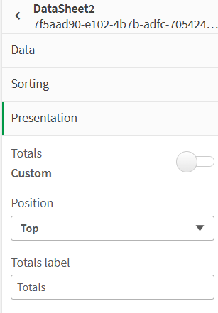
The Totals feature in each Data Section allows you to automatically calculate and display summary values for your measures — no extra formulas needed.

You'll find this option under the Presentation tab of the Data Section.

What You Can Configure:

1. Position — Choose where the totals row should appear:
   • None — No totals are displayed
   • Top — Totals row appears above the data
   • Bottom — Totals row appears below the data
2. Label — Set a custom text label for the totals row (e.g., "Total", "Summary", "All Regions")

   

Range

Ranges define specific target cells within a sheet where data from a hypercube's dimension or measure will be inserted. Instead of populating the entire sheet automatically, ranges allow precise control over where each data column starts.

For example, as shown in the configuration panel, you can bind a dimension to start from cell A2, while measures can be assigned to cells like B2, C2, etc.

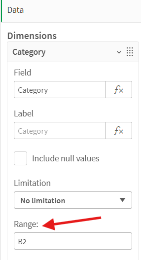
It is also possible to define limited ranges, such as B2:B10. In this case, only the top-sorted values from the hypercube will be displayed in the spreadsheet.

Additionally, you can specify horizontal ranges by entering a span like B2:J2. The values will be populated across columns instead of rows, and limited by the number of specified cells.

This approach enables embedding Qlik data into a customized spreadsheet layout while leaving space for charts, notes, or calculations around the data block.

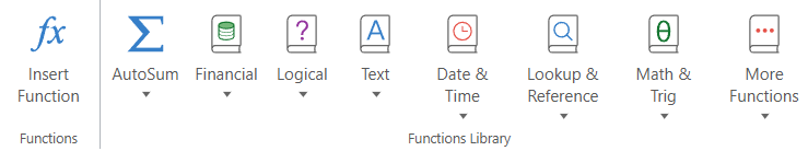
Excel Functions

The extension supports most native Excel functions, including:

• Math & Trig: SUM, AVERAGE, ROUND, INT
• Logic: IF, AND, OR, NOT
• Text: CONCATENATE, LEFT, RIGHT, TEXTJOIN
• Lookup: VLOOKUP, INDEX, MATCH
• Date & Time: TODAY, NOW, DATEDIF, EOMONTH
• Array: UNIQUE, SORT, FILTER

And many others.

Feel free to explore a full list of available Excel functions in the Formulas section of the Ribbon Menu.

Qlik–Related Functions

The Spreadsheets extension supports a set of Qlik–specific formulas that allow you to interact with data sections, extract values, labels, totals, or evaluate expressions directly in spreadsheet cells.

Each function runs asynchronously and returns dynamic values based on Qlik's associative model.

QLIK.DATA

Fetches and inserts data values from a preconfigured Data Section.

= QLIK.DATA(data_section_label_or_index, [column_label_or_index], [is_horizontal], [show_label], [show_total], [limit])

Arguments:

• data_section_label_or_index — Label or index of the Data Section.
• column_label_or_index — (Optional) Label or index of the column (dimension or measure).
• is_horizontal — (Optional) If true, data fills horizontally instead of vertically.
• show_label — (Optional) If true, includes column labels.
• show_total — (Optional) If true, includes total values.
• limit — (Optional) Maximum number of rows (columns if horizontal) to return.

Use cases:

• Embedding Qlik data into specific spreadsheet regions.
• Populating sheets with multiple datasets independently.
• Displaying data when automatic sheet–to–section binding is not desired.

QLIK.DATA.LABEL

Returns the label of a specific dimension or measure from a Data Section.

=QLIK.DATA.LABEL(data_section_label_or_index, column_label_or_index)

Arguments:

• data_section_label_or_index — Label or index of the Data Section.
• column_label_or_index — Label or index of the dimension or measure.

Use cases:

• Dynamically showing column headers.
• Building generic or reusable templates with flexible data inputs.

QLIK.DATA.TOTAL

Returns the total aggregation value for a specific measure in a Data Section.

=QLIK.DATA.TOTAL(data_section_label_or_index, measure_label_or_index)

Arguments:

• data_section_label_or_index — Label or index of the Data Section.
• measure_label_or_index — Label or index of the measure.

Use cases:

• Displaying total rows or summary KPIs outside the main data block.
• Referencing Qlik–calculated totals without manual summing.

QLIK.EXPRESSION

Evaluates a Qlik expression and returns the result.

=QLIK.EXPRESSION("=Today()")

Arguments:

• query_string — A Qlik expression wrapped in quotes (must start with =).

Use cases:

• Showing dynamic system values like date/time.
• Calling Qlik expressions independently of loaded data.
• Integrating master measures or global calculations directly into a layout.

Formatting

The Spreadsheets extension offers a comprehensive suite of formatting tools available in the Ribbon Panel, organized by sections. Below are the most frequently used tools from the Home tab, helping you quickly style and structure your spreadsheet content.

Home

Fonts: font size, color, bold, italic, underline, background fill, borders

Text Aligning: Vertical and horizontal alignment, Orientation, Indent, Wrap, Merge and Center

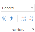
Number formats: currency, percentage, custom formats

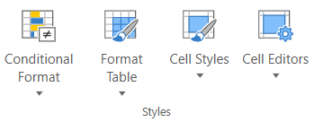
Cell Styling: Conditional Format, Table Format, Cell Styles, Cell Editors

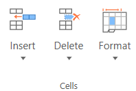
Cells: Insert, Delete, Format

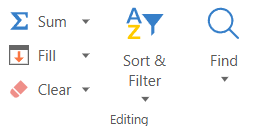
Editing: Insert Function, Fill, Clear, Sort and Filter, Find

Save / Load

All changes made within the Spreadsheets extension — such as entering static values, importing charts, applying formatting, or modifying data—must be saved explicitly to the app in order to persist.

There are two primary ways to save your work:

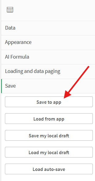
Option 1: Via Properties Panel

1. Open the Properties Panel.
2. Navigate to the Save section.
3. Click the Save to app button.

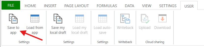
Option 2: Via Ribbon Menu

1. Go to the Ribbon Menu.
2. Under the User section, click the Save to app button.

Until changes are explicitly saved, your edits will exist only in the working session and may be lost on reload.

Import / Export

The Spreadsheets extension provides robust tools for importing and exporting data, enabling smooth interaction with external files and software

Importing Excel or CSV Files

To import data, open the FILE tab in the ribbon menu and select Import. You can upload either an .XLSX (Excel) or .CSV file.

Each import type includes a set of configurable options that control how the file is processed. Depending on the selected format, you may be able to preserve formatting, formulas, merged cells, calculation settings, and more. These options ensure that imported content behaves and appears as expected in the Qlik environment.

Once imported, the spreadsheet maintains its structure and styling, making it easy to continue working with existing data or templates. You can also enrich the imported file with Qlik–driven charts, additional sheets, or calculated logic.

Exporting to Excel, CSV, or PDF

To export your spreadsheet, go to the FILE tab and choose Export. You can save the current workbook in .XLSX, .CSV, or .PDF format, depending on your needs.

Each export format includes its own configuration panel, allowing you to tailor the output. For example, you may choose to include styles, formulas, layout elements, headers, or control how merged and empty cells are handled. These options help ensure your exported document preserves the desired structure and content fidelity.

AI Formula

The AI Formula feature allows you to run natural language queries using a connected AI model (in alpha version supports connection only with OpenAI). This enables spreadsheets to become interactive, intelligent tools — capable of generating or transforming content on the fly using language–based prompts.

Configuration (Property Panel)

To use AI formulas, go to the AI Formula section in the properties panel of the extension and configure the following settings:

• AI server URL — The endpoint for the OpenAI API (e.g., https://api.openai.com/v1/chat/completions)
• AI model — Currently supports:
  • Gpt–3.5–turbo
  • Gpt–4
  • (Additional models will be added in the future)
• Max tokens per request — Controls the length of the AI's response (default: 4000)
• Formula evaluation mode — Determines when the AI is queried:
  • On recalculation
  • Once
  • On interval
• API Key — Your OpenAI secret key (must have valid access rights to the selected model)

Using the AI() Formula in the Spreadsheets

Once the above settings are configured, you can use the following formula directly in spreadsheet cells:

=AI("Translate this sentence to Spanish: " & A2)

Formula Syntax:

AI(query_string)

• query_string — A string prompt that will be sent to the selected model (can be static or dynamic using cell references)

The result will be displayed directly in the cell where the formula is entered.